Introduction

Welcome to my latest blog post where we will be discussing the recent paper “A Long Short-Term Memory Network for Plasma Diagnosis from Langmuir Probe Data”. This paper, published in the Journal of Nuclear Materials and Energy, presents a new approach to diagnose plasma using a Long Short-Term Memory (LSTM) network. As a fusion physicists, I am always excited to see new techniques and ideas being applied to the field of plasma physics. In this post, I will provide an overview of the paper, explain what an LSTM network is and how it works, and give some thoughts on the potential impact of this research on the fusion field. So, let’s dive in!

Fusion plasmas… why are they important?

The development of fusion plasma devices has rapidly increased in the last 20 years, bringing us ever closer to green, sustainable energy. Plasmas as the fourth state of matter where ions and electrons are unbound and move freely from one another at high temperatures. These high temperatures and pressures maintained by various heating techniques and supercooled magnets cause nuclei to fuse, generating massive amounts of energy. However, maintaining a fusion plasma is no easy task. Safe ignition, maintenance, and dispersion of plasma discharges are heavily reliant on the capabilities of the diagnostic sensors. As the majority of small to medium sized reactors only produce plasmas for 0.001-1 second, diagnostics must be fast, responsive, and accurate to provide live feedback control or accurate post-plasma diagnostics. Plasma parameters such as electron temperature, density, and potential are calculated from data collected by these diagnostic sensors. These parameters are vital for determining the state of the plasma; whether the plasma is stable or tending to instability etc.

Langmuir probes are a commonly used method for diagnosing the parameters of a plasma. They involve active and indirect measure of the plasma and in this case, the plasma is changed in a small area by the probe to obtain the characteristics from it. However, the calculations required to extract the plasma parameters typically have to be done manually post-experiment, which limits the ability to use Langmuir probes as a real-time diagnostic tool. Various external factors (such as probe surface area) can also impact the accuracy of the plasma measurements obtained through Langmuir probes, which can make the data messy and hard to fit using traditional methods.

The work of authors et al. aims to create a more universal, robust, and accurate method of plasma diagnosis by speeding up parameter calculations and eliminating the influence of external factors using long short-term memory (LSTM) recurrent neural networks (RNN).

The Langmuir probe and how it works

Langmuir probes, proposed in 1926, are a commonly used diagnostic tool in plasma physics research. They essentially work by inserting a small probe into the plasma, collecting electrons and measuring the electrical characteristics of the plasma at that point. The probe has a small wire or needle that is oscillated between being positively and negatively charged, which is inserted into the plasma. The electrons in the plasma are attracted to the positively charged probe and flow toward it, creating an electric current. By measuring the current as a function of the voltage applied to the probe, we can deduce important properties of the plasma from the I-V characteristics, such as the electron temperature, $T_e$ and density, $n_e$. One of the great things about Langmuir probes is that they can be used to make measurements in a wide range of plasmas, from fusion plasmas to the plasma in space. They are a simple yet powerful tool that can provide a lot of information about the plasma being studied [1].

How are I-V characteristics calculated?

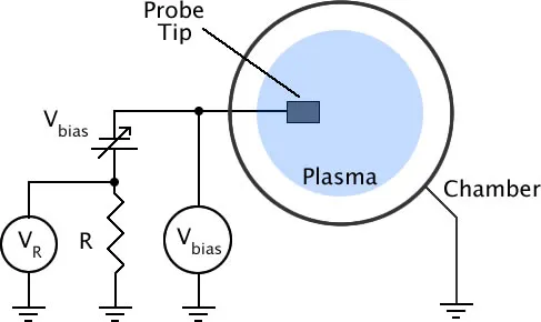
Figure 1: Circuit diagram of the Langmuir probe setup

The aim of the paper is to determine the characteristics $n_e$ and $T_e$. These are found using theoretical models based of a perfect plasma and fitting them to the data obtained from the probe. The perfect data curve from a Langmuir probe would look a little like an ‘S’ like that in fig. 2. For those interested in how Langmuir’s method classically fits the data and finds the characteristics, we go into a little more mathematical detail here, otherwise feel free to skip to the next section Problems with measurements.

I-V characteristic is obtained by sweeping a bias voltage (VB) from negative to positive potentials. From these curves the plasma characteristics are calculated from specific features of the curve:

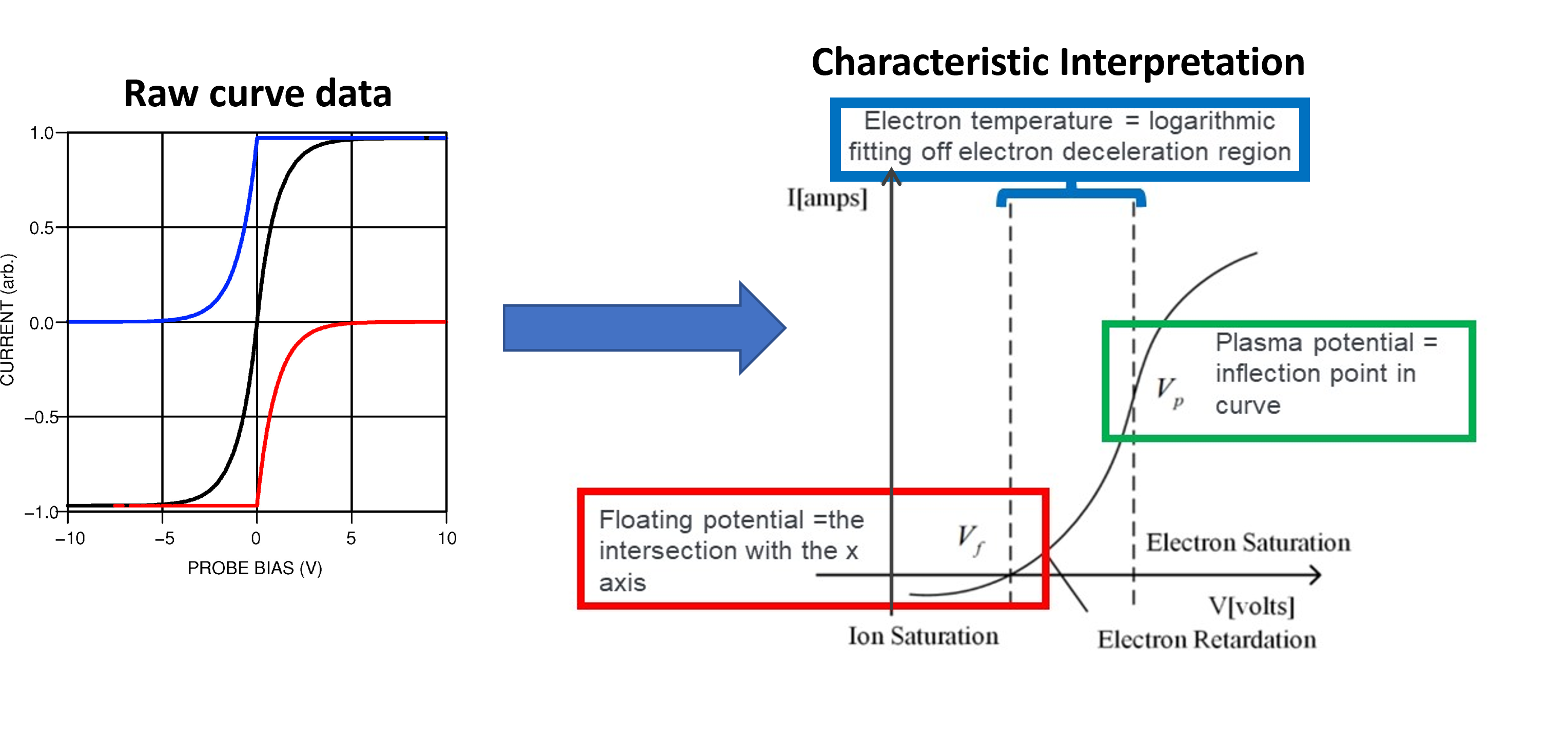
Figure 2: Langmuir probe I-V characteristic

The total current in fig. 2 is represented by the black curve and the ionic and electron current are represented by the blue and red curves respectively. Different features of the black I-V characteristic are used to find $n_e$ and $T_e$:

• Floating potential, $V_f$: The point where the total voltage of the probe changes sign
• Plasma potential, $V_p$: The point where the curve bends to the right (i.e. Where all the electrons are repelled)
• Electron temperature, $T_e$: The gradient of the middle region labeled in blue on fig. 2 is $=e/{(k_bT_e)}$

Knowing all these values allows us to apply the following relations to determine $n_e$ using,

Where the new terms here are ion mass, $M$, area of the probe, $A_s$ and the physical constants, $k_B$ = Boltzmann’s Constant and $e$ = electric charge.

These Characteristics are obtained post-processing, and curve fitting of the data collected during experimentation. These relations are purely based on theory, and change depending on the probe geometry, conductivity, plasma type, etc. In most cases, these relations are taken and fitted with additional constants to compensate for these effects and can be a very lengthy process, as each curve needs to be fitted individually.

Problems with measurements

Theoretical models are seldom perfect and the case of Langmuir probes is no different. The I-V characteristic drastically deviates from the standard form if the surface layer of the probe is contaminated or if the probe is placed in a low-density plasma. The characteristic bends in the curve are no longer as obvious, and as the voltage oscillates between negative and positive, the current, (I) values no longer overlap. This can make the gradient value very hard to find. An example of the effects of contamination and low density can be seen in fig. 3.

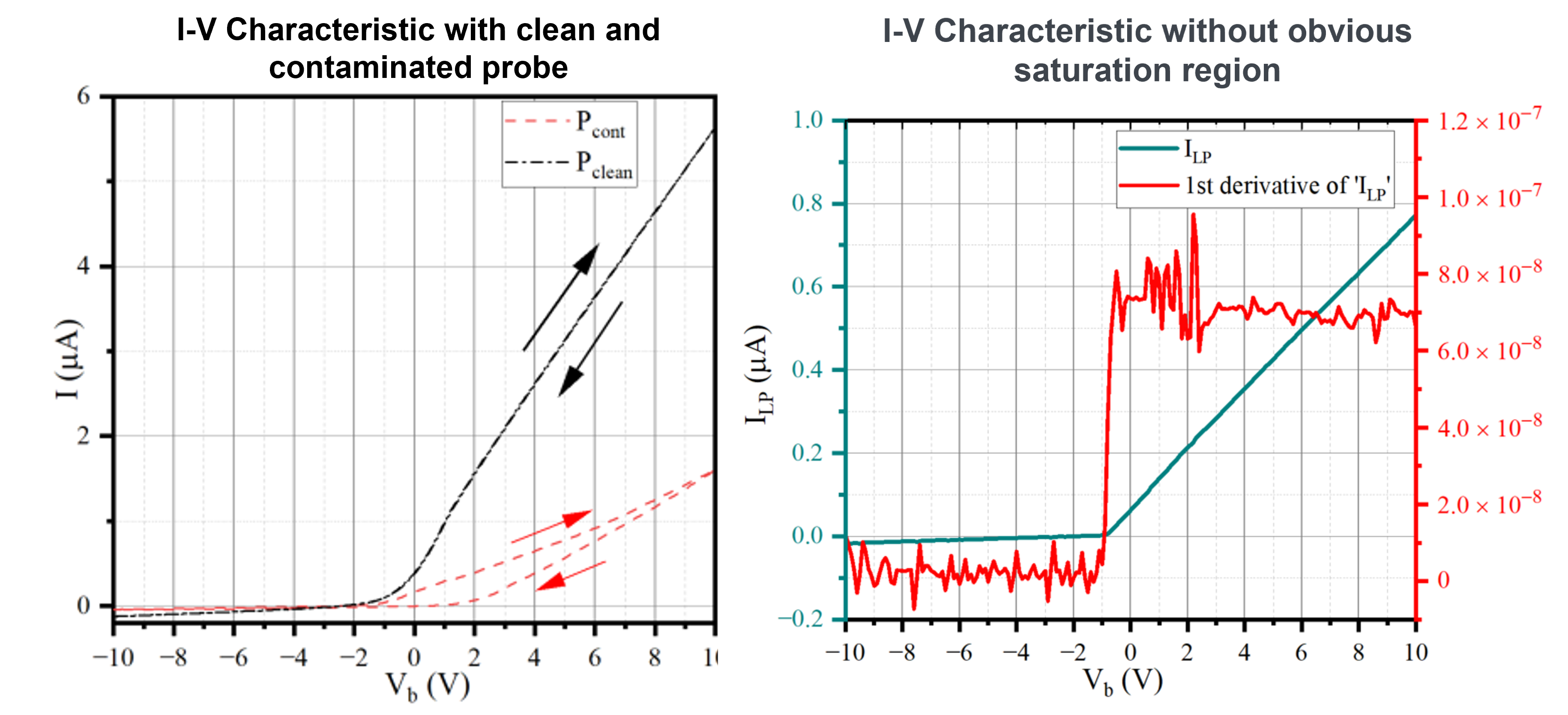
Figure 3: A contaminated probe's I-V characteristic compared to a clean probe's (Left) and a low density plasma I-V characteristic (Right).

Contamination results in the curves no longer coinciding when the voltage oscillates between negative and positive. Low-density plasmas result in a very high SNR as not as many electrons are collected. This results in messy data and no intermediate region where the logarithm can be fit.

Faced with these issues, traditional fitting methods can be even more of a challenge. Different levels of contamination and low data acquisition of low-density plasmas leads to a lot of noise in the data. Hence, each curve needs to be manually fit on a case by case basis. This process requires a lot of computational resources and can be very slow, which isn’t ideal when you’re trying to analyze data in real-time. So, the goal of this research was to develop a new method for diagnosing plasmas using Langmuir probe data that is faster, more accurate, and doesn’t suffer from the problem of probe contamination and low-density plasmas. And, it looks like they succeeded!

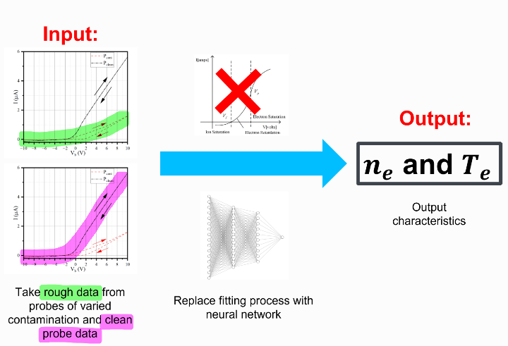
Figure 4: The authors goal for the architecture their network.

Background on Machine Learning

Predicting $n_e$ and $T_e$ is a simple regression problem and can be resolved with a simple multi-layer perceptron (MLP) network. These MLP networks are relatively easy to use and lightweight, but are not suited to characterize the messy data that could be affected by multiple factors of varying degrees (such as the level of contamination). Hence, instead of using a one-way propagation system in the MLP, they use a neural network structure called long short-term memory network.

LSTM , what is it and how does it work?

Now hopefully, when I mention Langmuir probes again, you have a general idea of what I’m talking about. This is because we don’t start thinking from scratch. All because we have moved on to the next section, doesn’t mean we forget everything from before. As you read the blog, you understand the context of each section based on the previous sections. You don’t throw away all your knowledge and start thinking from scratch again. There is a certain continuity to our thoughts.

However, traditional neural networks can’t do this. Regular neural networks have a hard time understanding sequences of data. They’re good at recognizing patterns in a single data point, like identifying a picture of a cat… as a picture of a cat. But when it comes to understanding something like a sentence or a time series, regular neural networks can struggle. Sequential networks struggle relating previous words in a sentence with the next ones, essentially, forgetting everything every time new information is given. Recurrent neural networks (RNNs) attempt to solve this by having loops within the network, allowing them to persist. RNNs can be thought of as multiple copies of the same traditional sequential network but every time it runs, information is carried over to the successor.

Because of RNN’s ability to remember past information, they have been incredibly successful when applied to tasks such as translation, text generation, speech recognition… and many more.

However, RNNs have some fatal flaws and may not be completely suitable for prediction based on information given quite a while ago. This was explored in detail by Hochreiter, who proved mathematically to why this is difficult.

That’s where LSTMs come in. LSTMS are a special kind of RNN used for any series where a sequential prediction is required, and long-term dependency is attached to it. Like all neural networks, there are repeating cell with hidden layers (e.g. activation function) side. The LSTM cell looks like this:

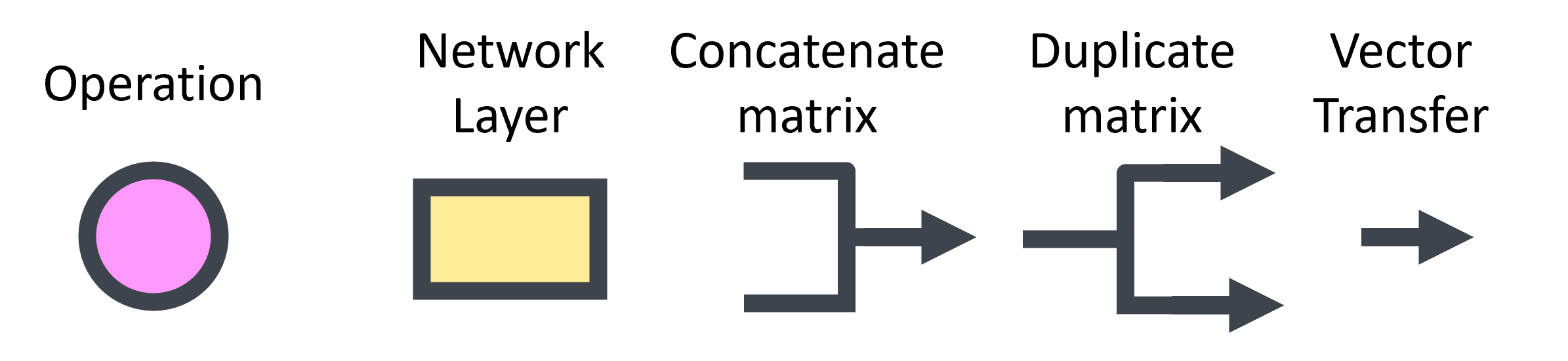
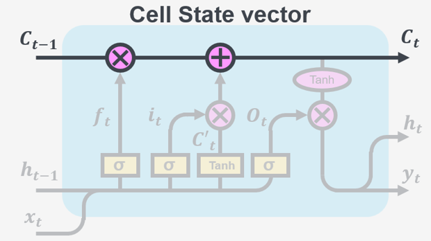
Figure 5: A general structure of an LSTM cell.

The diagram above illustrates how information flows through an LSTM cell. Each line represents a vector that connects the output of one node, to the input of others. The pink circles represent simple operations like adding vectors together, while the yellow boxes represent activations. When lines come together, it means the vectors are being combined, and when a line splits, it means the information is being copied and sent to different parts of the LSTM cell.

To understand exactly what an LSTM cell is doing with the data, lets break it down into 4 parts.

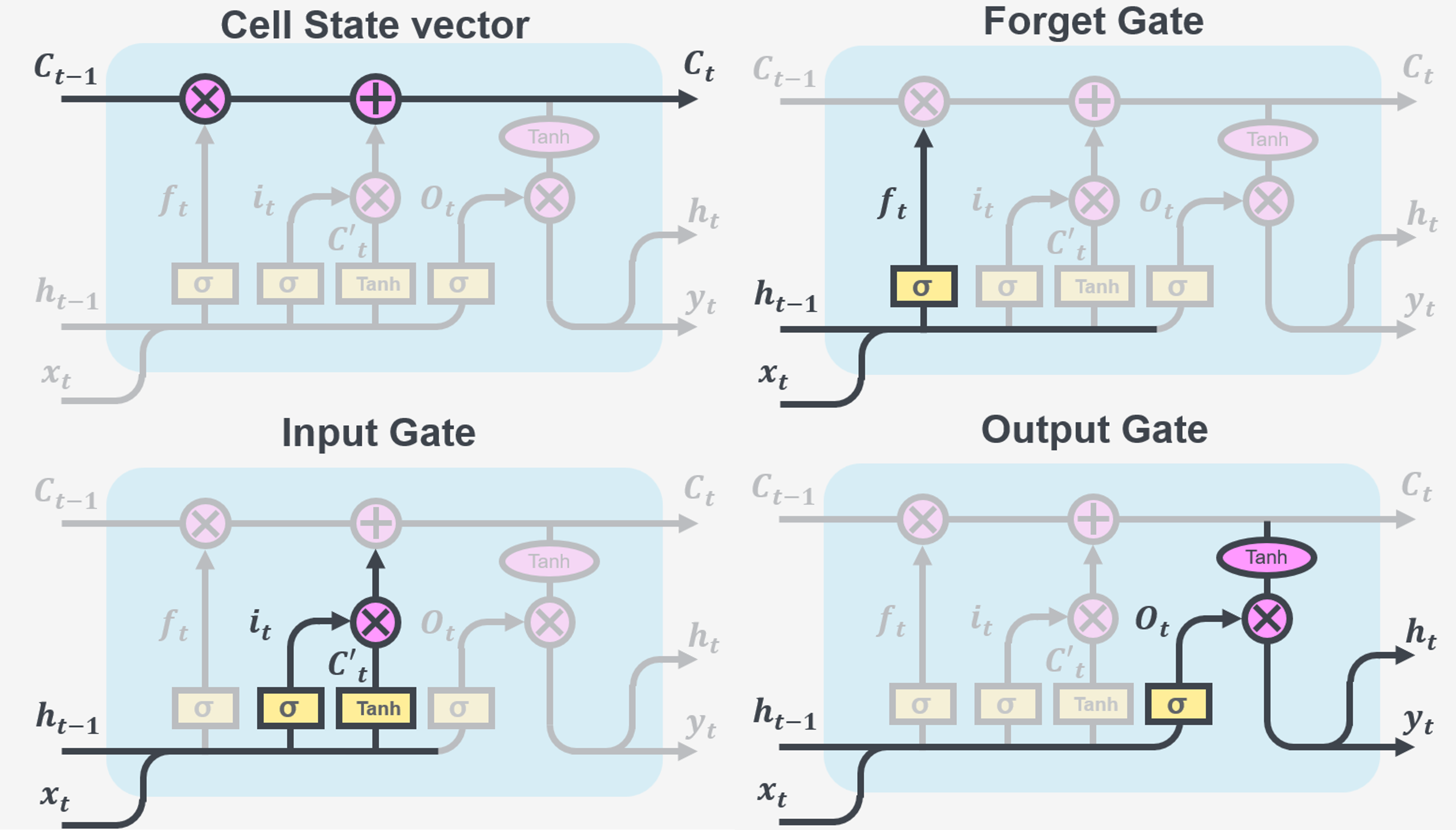
Figure 6: A breakdown of an LSTM cell.

The memory part of the LSTM cell is the cell state vector. Information is added or removed to the cell state via the interactions with the gates. Gates consist of two parts: a sigmoid activation and a point-wise multiplication operation. The sigmoid activation is used to decide how much information should be kept or discarded (by assigning a value between 0-1), and the point-wise multiplication operation add this information to the cell state.

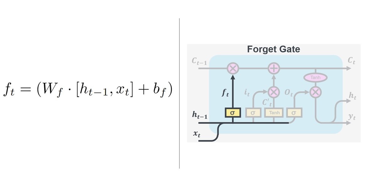
The first gate controls how much information we want to remove from the cell state, hence aptly named the ‘forget gate’. It takes the output value $h_{t-1}$ from the previous cell and the new data point $x_t$ and decides how much information from the previous cell is relevant. Combining that with the trainable weights, $W$ and biases $b$ of that layer results in $f_t$ being passed onto the cell state vector. $f_t$ is multiplied by the old cell state, $C_{t-1}$ hence the cell forgets what it has decided to forget and is passed onto the next gate.

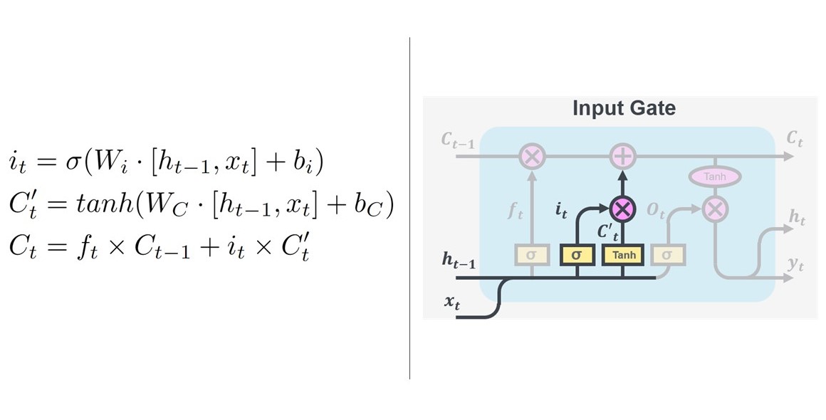
Now its time do decide which information from the new data is doing to be passed on to the cell state. This is determined by the ‘input gate’. The sigmoid activation chooses what to keep and what needs updating and the tanh activation creates a vector of suggested new values for the update, $C_t’$. Now that we have what needs replacing and what we could be replaced with, again, we update the old cell state, $C_{t-1}$ by $i_t \times C’_t$ to the new cell state $C_t$. This updates the chosen cell haves from the sigmoid activation.

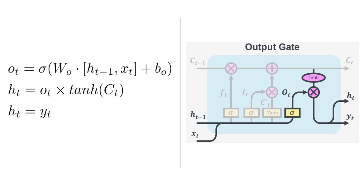
Finally, we decide what we want to output from the cell, determined by the output gate. The output gate combines the cell input $h_{t-1}$ with a modified copy of the new cell state $C_t$. This means only the important parts of the cell state and previous cell are kept and passed on as the new input to the next cell, $h_t$. This output, $h_t$ is then copied and outputted at $y_t$.

These cells can be strung together and are great for time-dependant data and memory tasks. Now we have a better idea of whats going on in the cell, we can look at how the paper applies LSTM networks to the Langmuir probe data.

If you’re interested in how LSTMs work in detail and want to know how different types work, I would recommend reading colah’s blog from which I took inspiration for my explanation.

Experimental setup

Collecting data

In this experiment, we’ll be looking at the effects of humidity on two identical Langmuir probes - one labeled “Pcont” and the other “Pclean.” First, we’ll leave both probes exposed to a humid atmosphere for more than 24 hours, thus ‘contaminating’ them. Next, we’ll place both probes on a special platform in a plasma vacuum chamber and mark their positions. They are placed the same distance away from the plasma course, so that they will detect the same plasma conditions.

Then, we’ll heat up a filament and fill the chamber with argon gas to create a steady plasma discharge. We’ll apply a negative 200V to the Pclean probe for ten minutes to remove any contaminated layer on the probe’s surface by heating it and using electrons to bombard it.

After that, we’ll use the platform to move both probes to a central position and collect data on their current and voltage (I-V) characteristics. We’ll make sure to collect data on both probes within a one-minute time frame.

Finally, we’ll analyze the collected data using both traditional diagnostic methods and the LSTM network. This will allow us to compare the results and see how well the advanced technique performs.

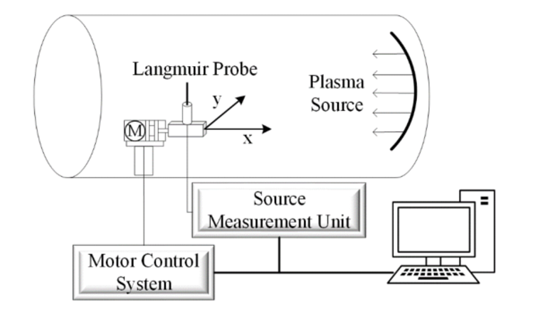
Figure 7: Diagram of the experimental setup.

Why do we actually need LSTM

When we apply these traditional fitting methods to contaminated probe data, we usually get very poor results. The methods that are applied to the clean probe data are the same applied to the contaminated probe and then fitting parameters are iteratively added to try and recover the correct result. Essentially, we ‘remember’ the clean probe data and use traditional fitting to get our $n_e$ and $T_e$ and then (under the same plasma conditions) try to make the contaminated probe data fit the same $n_e$ and $T_e$ by tweaking the math we saw in section The Langmuir probe and how it works. Additionally we don’t actually know by how much the probe is contaminated, so each measurement need to be treated separately to try and calculate a meaningful result.

The LSTM network does exactly the same thing: by remembering the result of the clean probe in the same measurement, it is able to find the relation between the contaminated probe data and the clean probe data, thus predicting the temperature, $T_e$ and density, $n_e$. As the network can learn what a clean vs.contaminated probe’s I-V characteristic looks like, w when they are given a new contaminated probe’s data, it relates it to a clean probe’s data under the same conditions and gives out more accurate $n_e$ and $T_e$ predictions. This gives a more general model and each fit is done automatically rather than manually.

Network structure

Now we move onto how the network in this paper is trained and how they went about making sure the LSTM model was the best fit to the data. Using two blocks of the LSTM cells from section LSTM, what is it and how does it work?, a two layer LSTM model is built. However, using a two-layer LSTM network can sometimes cause something called “overfitting,” which means the model is too complex for the data it’s working with. It picks up on small data patterns such as noise rather than the overall shape of the data (which is what we know is used to calculate the $T_e$ and $n_e$). To avoid this, we’re adding something called a “random deactivation layer” after each layer of the LSTM network.

A random deactivation layer helps to prevent overfitting in the LSTM network by randomly deactivating or ‘dropping out’ some of the neurons during training. This serves to reduce the complexity of the network and make it less likely to memorize the training data and the small details that the network could pick up on as patterns.

The idea behind dropout is that it prevents neurons from co-adapting too much. In other words, it helps to break the inter-dependency among neurons, which makes the model less sensitive to the specific weights of neurons. By randomly dropping out neurons during training, we force the network to find different ways to solve the problem, look for more general correlations in the data, and increase robustness, which helps to reduce overfitting. This results in a more generalizable model, which is better able to generalize to unseen data.

Finally, they added something called a “fully connected layer” to the network, which will help the network output values that match up with the actual data. They compared the output values of the network to the actual data, and use a specific algorithm called Adam optimiser to update and improve the model’s parameters.

To summarise, they used the model structure seen in fig. 8 to try to find the best way to improve the model without overfitting to the data.

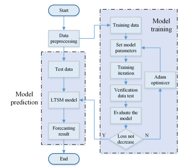
Figure 8: Diagram of the network setup.

Results

Data

After processing all the data using traditional methods, the authors obtain a dataset of 5186 groups. $n_e$ ranges from 1012 to 1014 $𝑚^{−3}$, $T_e$ ranges from 19,000 to 60,000 K and current ranges 70 A, 80 A, and 85 A. Changing the current to lower values, decreases the density of the plasma. So, they created a large data set in a broad parameter space.

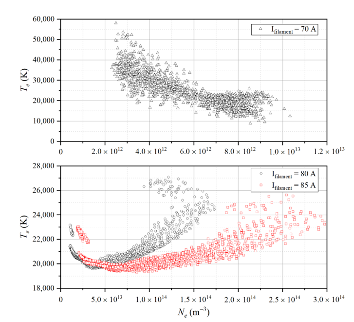
Figure 9: All data obtained using traditional processing methods

This data set was split into 4150 samples for training and 1036 samples for testing.

Optimising hyperparameters

When working with a neural network, there are many different parameters you can adjust to improve the performance of the model. These can include things like the number of neurons in each layer, the number of layers, the learning rate and so on… In most cases with neural networks, this training is mostly a trial and error as the process of finding the optimal hyperparameters for a neural network can be challenging as it depends on the complexity of the problem, the size of the dataset, and the architecture of the network. In this specific case, by adjusting these parameters, they were able to fine-tune the model to give the best possible predictions. The researchers are using the accuracy of the prediction of $n_e$ to adjust these parameters and find the best structure for their neural network.

Evaluation indicators

When it comes to training a machine learning model, it’s important to have a way to measure how well the model is performing. This is where evaluation indicators come in. Evaluation indicators are metrics used to measure the performance of a model, and they can help you understand how well the model is making predictions.

In this specific case, the researchers are using two different evaluation indicators: the mean square error (MSE) loss function and the mean absolute percentage error (MAPE).

The MSE loss function is a common metric used in multi-output regression prediction models. It calculates the difference between the predicted value and the actual value, and it’s usually used to measure the accuracy of the model during training. It’s sensitive to large differences between the predicted and actual values hence, during training the model will change its parameters more if the MSE is large.

After the model has been trained, the researchers are using the MAPE metric to evaluate the performance of the model. The MAPE calculates the percentage difference between the predicted value and the actual value. A percentage error helps to give a more intuitive understanding of how well the model is performing.

Neuron density

The number of neurons in a layer can drastically change how your network learns. Too may neurons and we may over-fit the data and too few and the neural network may not pick up on the patterns in the data. The researchers varied the number of neurons tested for the network’s predictive accuracy. Among them, the network with the 50R4/4/1 structure can achieve a higher accuracy faster. This can be seen in fig. 10 where the 50R4/4/1 clearly peaks in accuracy well before the other network structures.

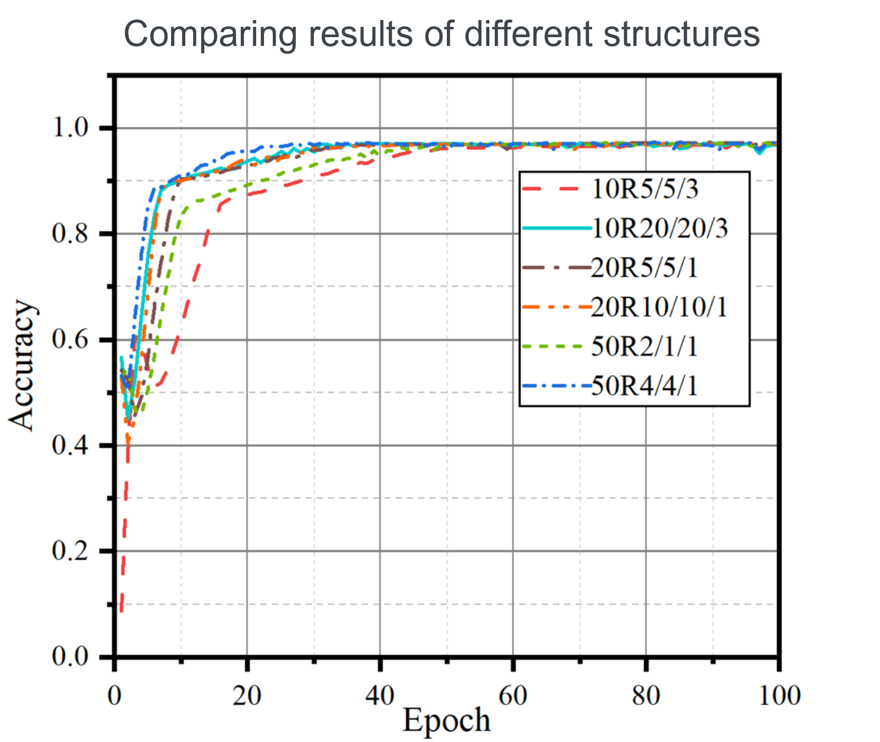
Figure 10: Different model structures tested for prediction accuracy of $n_e$.

50R4/4/1 in the researchers notes means: 50 $\times$ 4 = 200 neurons in the first layer, 50 $\times$ 4 = 200 neurons in the second layer, and 50 $\times$ 1 = 50 neurons in the Full connection layer.

Learning rate

When it comes to training a neural network, one of the most important things to consider is the learning rate. The learning rate is a hyperparameter that controls the step size at which the optimiser makes updates to the model’s weights and biases during training. In other words, it determines how fast the model learns. Imagine you’re on a hill and you want to find the best path to take to reach the bottom. If you take too large steps you may miss detail along the way, if you take too small steps, it may take too long to reach the bottom. This works the same way for the optimiser. A high learning rate means that the optimiser is making big jumps in the weight space and can cause the model to converge too quickly to a suboptimal solution or diverge. On the other hand, a low learning rate means that the optimiser is making small steps and can cause the model to converge too slowly to the optimal solution. Finding the sweet spot between these two extremes is crucial to make sure the model is learning efficiently and effectively. In this case, the researchers used various fixed learning rates to see which worked best, of which 0.00001 was the best with lowest RMSE and MAPE.

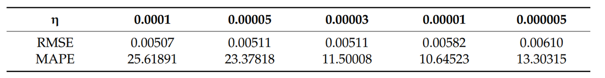
Figure 11: Testing for different learning rates.

Loss and Accuracy

The loss and accuracy plots for both $n_e$ and $T_e$ seen below in fig. 12 show that the researchers were able to achieve a 95% accuracy within 50 epochs.

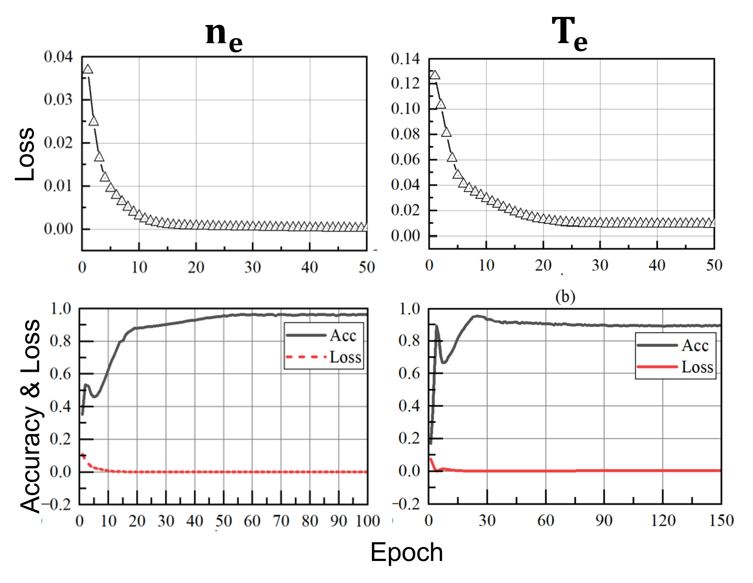
Figure 12: Looking at the loss and accuracy of predicting $n_e$ and $T_e$.

They state that they optimised the network hyperparameter structure from just the accuracy of the prediction of $n_e$. I question their choice of method here. Although they are training the model based on the accurate prediction of more than one variable, optimising the structure based on one makes it seem like they’re leaving the prediction of $T_e$ down to a lucky guess, rather than a network that models the whole system. Although you can see a relatively high prediction for both $n_e$ and $T_e$, the prediction accuracy for $T_e$ is a few percent lower and the loss function does not converge as well as for $n_e$.

The researchers suggest that the benefit of using an LSTM network for plasma diagnosis lies in the lack of coupling between the acquisition of Ne and Te. This eliminates the potential impact of significant errors in Te on the result of Ne, which is a common issue in traditional diagnostic methods. I would disagree with this statement. With a network structure optimised to predict only one of the two variables better, the network may be using the prediction of $n_e$ to influence its prediction of $T_e$. Hence their prediction may not necessarily be completely decoupled.

Prediction

Using the now trained and tested LSTM network the researchers predict $n_e$ and $T_e$ from contaminated probe data and see if they can eliminate the effect of contamination from plasma diagnosis data. In fig. 13, we see the comparison of the characteristics calculated using classical methods from the clean probe (Ground Truth) in blue, the contaminated probe in grey, and the LSTM prediction in red. Looking at the trends in the data, the contaminated probe seems to under-predict $n_e$. The LSTM almost finds a middle ground between the clean and contaminated probe data, raising the value to $n_e$ to best match that of the clean probe. Hence, when we compare the error between classical methods and the LSTM model for finding $n_e$ the error decreases by 25%!

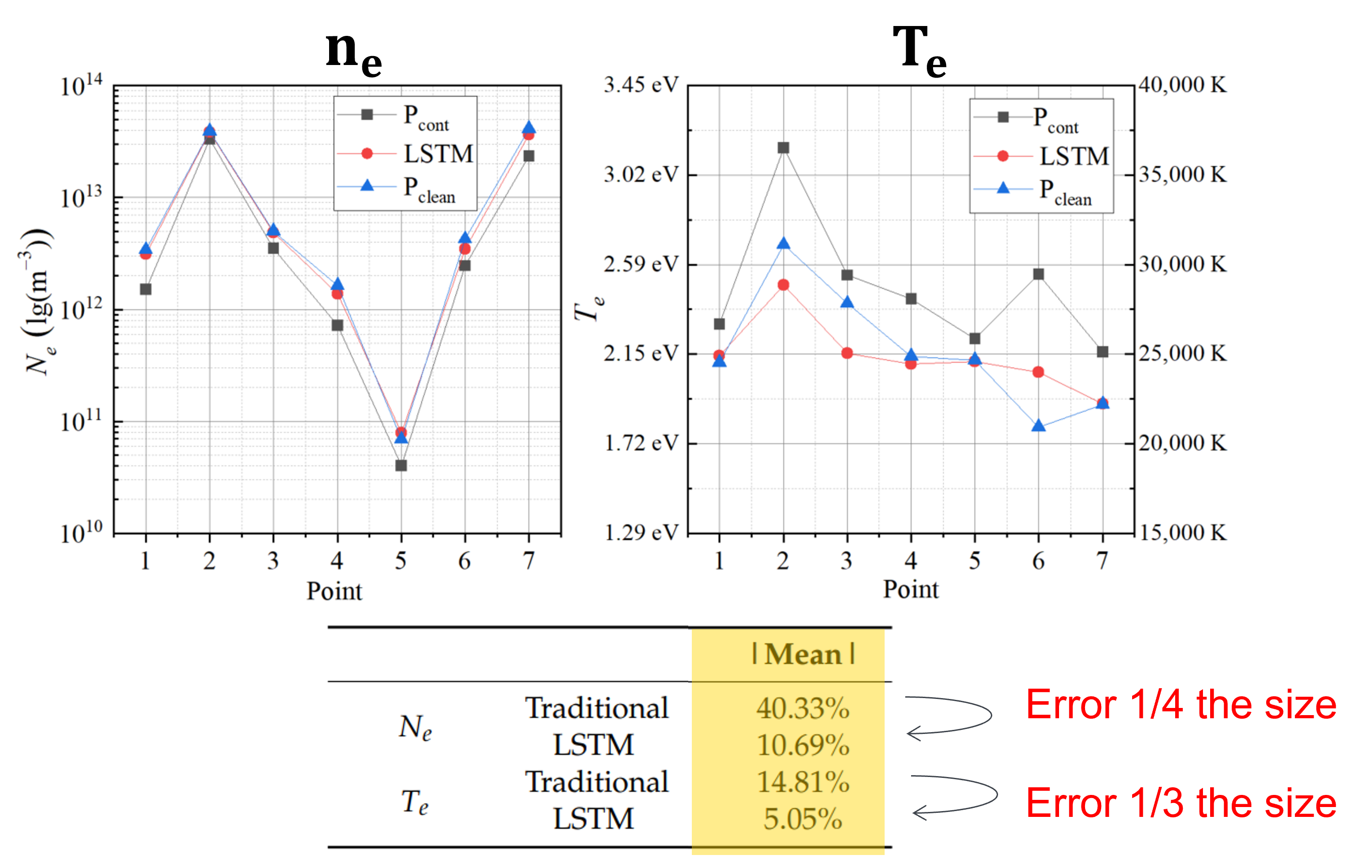
Figure 13: Comparing the clean, contaminated, and predicted data from the Langmuir probes for $n_e$ and $T_e$.

Despite the error decreasing by 30% for $T_e$, when we look at the graph for $T_e$ we can see that the LSTM is not exactly finding the right pattern. Opposite to the prediction of $n_e$, the effect of contamination on the classical calculation of $T_e$ results in an overestimation. The LSTM seems to over-predict the $T_e$ value, not quite matching the trend of the clean probe data. I can only assume this is because the hyperparameters of the network were optimised on the prediction accuracy of $n_e$, not $T_e$, however the researchers argue that:

This problem seems to need more $T_e$ data with a larger distribution range to train the network.

In the case of under-dense plasma, the researchers make the the argument that inaccuracy of traditional methods and the small amount of data in the low density region resulted in low prediction accuracy of the low density region by the LSTM. This is because the calculation process of $T_e$ requires logarithmic fitting of the electron retardation region of the I-V characteristic curve, which can be difficult to achieve in under-dense plasmas, hence the large amount of noise in the classically calculated $T_e$. The limitation of these traditional methods in turn, makes it difficult to use the data to train and predict from the LSTM network. As seen in fig. 14, both the prediction of $n_e$ and $T_e$ at low density (70A) is not as accurate as higher density, especially for $T_e$. The researchers a argue that:

The main reason for the poor accuracy of network prediction in the underdense plasma environment is that the calculation results of $T_e$ by traditional diagnostic methods are relatively inaccurate.

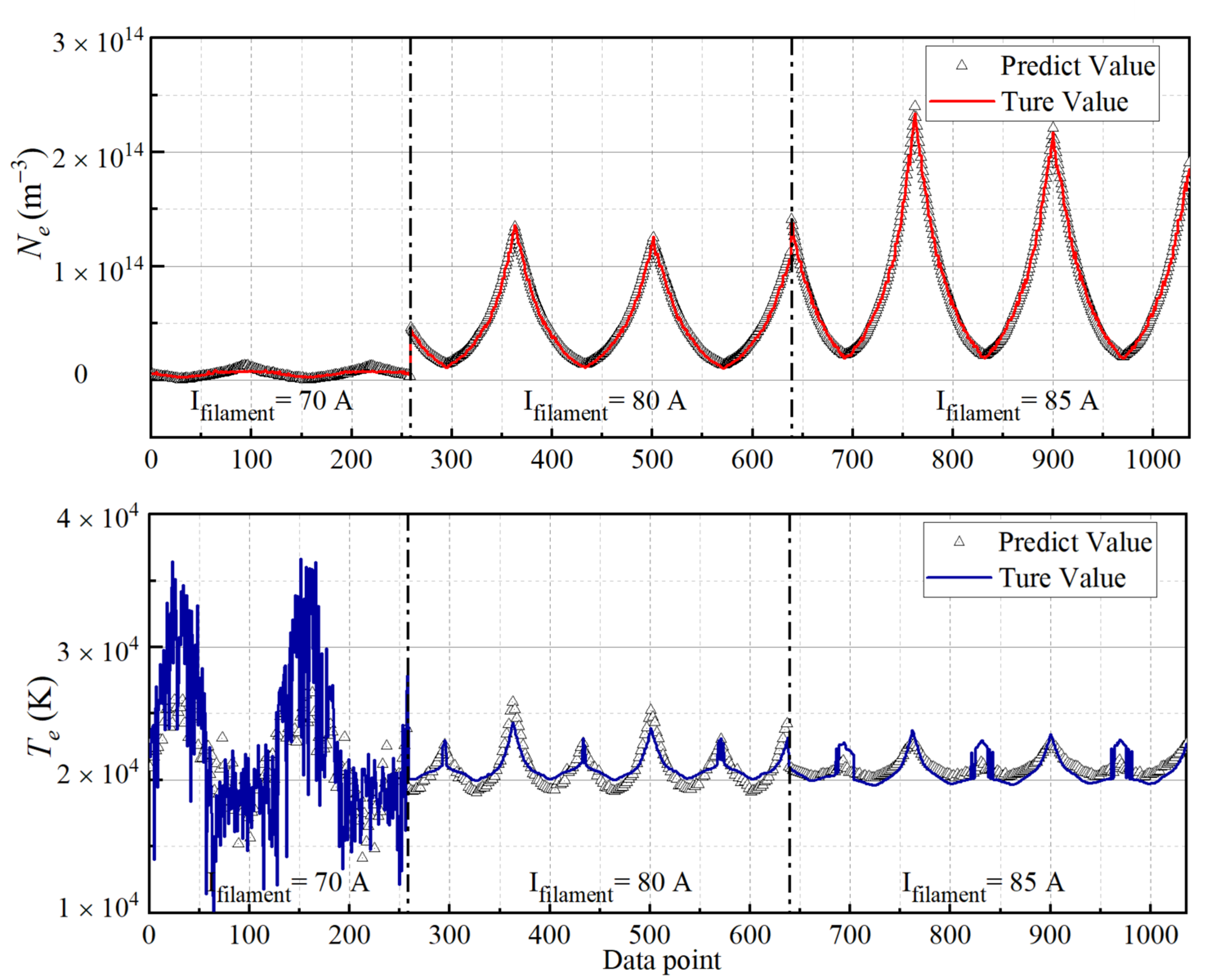
Figure 14: Comparison of $n_e$ and $T_e$ prediction in low and high density plasmas.

Conclusions

In summary, the use of an LSTM network proved to be an effective method for eliminating contamination and improving the accuracy of plasma diagnoses. By removing the effect of contamination on the probe data, researchers can receive more reliable results and gain a deeper understanding of the plasma’s properties, even when the probe is contaminated. The LSTM method only needed 10% of the data points for accurate LSTM $n_e$ and $T_e$ prediction when compared to traditional methods. This is a huge advantage! Less data means measurements can be made for less time and overall more measurements can be made without compromising on the accuracy of the calculated plasma characteristics.

When predicting $n_e$ and $T_e$ for under-dense plasmas, the researchers argue that not only are traditional methods inaccurate but also there is a significant lack of data in this region to efficiently train the network. Nevertheless, their model performed well at normal density.

Review

Overall, the researchers have created a new way of predicting plasma characteristics accurately and efficiently. However, in my opinion (and theirs too), there are some improvements that could be made to better predict $T_e$. Optimising the hyperparameters of the network based on the accuracy of both $n_e$ and $T_e$ or another metric such as the MAE would be a better fit to a multi-continuous-output problem.

Although the researchers made the argument that using an LSTM network essentially decouples the prediction of $n_e$ and $T_e$, reducing the error usually propagated through the classical fitting model. I would argue that the LSTM network would be able to find this coupling in the pattern of the data and still cause exactly the same problem. This is because, the two parameters are physically and mathematically linked by the physical parameters of the plasma experiment. As neural networks are trained to pick up on patterns in the data, I can’t say for sure that the patterns used to predict $n_e$ are decoupled from those to predict $T_e$ within the same network. As the network is more or less a black box to someone who doesn’t have access to the code, I cannot back this argument with data, but neither have the researchers.

The prediction in under-dense plasma, in my opinion, should have been made by a separate model specifically trained for under-dense plasma. The relations between clean and contaminated probe data and under-dense plasma together cover an extremely broad parameter space. Especially in the case of under-dense plasmas the probes are more vulnerable to sheath and edge charge effects, which affect the data differently to the contamination problem. The SNR is also a lot higher as there aren’t as many electrons in the plasma and therefore not as many are being collected. In addition, the researchers do not separate the prediction of clean and contaminated probes for under-dense plasmas. Here, it is difficult to tell whether there is an improvement to the classical model compared to the LSTM model. I would suggest separating the two problems: use unsupervised learning for predicting parameters at low density without contamination and improve the current LSTM to predict $n_e$ and $T_e$ from contaminated probes.

Following the low density problem, another point that the researchers argue is that $T_e$ in underdense plasma is inherently difficult to predict using classical methods as the logarithmic curve cannot be fit well, resulting in a very large error in the calculation. They use this an argument to defend why their predictions of $T_e$ with the network are not as consistent at $n_e$, but I don’t believe this is the case. I think,we are left with the classic ML problem of rubbish in, rubbish out. The network will train on these inaccurate values and be rewarded for getting closer to the inaccurate values. If the traditional fitting methods are not accurate enough, we could use unsupervised learning model to either cluster or associate the curve shapes with particular parameters, and calculate $T_e$ from that. Then, if contaminated probes were to be used in low-density, the unsupervised model could be paired with a more tailored LSTM to also predict $T_e$.

Finally, an interesting addition to this study could be to add a prediction of the level of contamination to the network. Contamination affects the shape of the data and that effect could be measured. This could be used to improve current classical models and identify contamination where it is present.

Acknowledgments

I would just like to say thank you to both Mathias Niepert and Mario Kalimuthu at the University of Stuttgart for running this seminar on machine learning in the sciences. Their course has been a very useful to approach ML in a more practical and enjoyable way. Special thanks to Mario for spending hours helping me get set up with Markdown and Git!